
If you’ve been watching Ontario’s electricity costs closely over the past few months, you may have noticed something that doesn’t quite add up.
In January and February, most of Ontario’s businesses (Class B) paid very high commodity rates as well as positive Global Adjustment (GA) rates – despite the fact that actual system GA costs were negative in those months. Then, in March, everything flipped. Commodity dropped to roughly 4.5¢/kWh, GA came in at approximately -4¢/kWh, meaning that the total landed at just ~0.5¢/kWh.
Meanwhile, larger Class A businesses experienced something very different. They paid the same high commodity rates in January and February, but their GA was already negative. Then, in March, while commodity fell, their GA turned positive.
Taken at face value, this looks inconsistent. Why would two groups, paying for the same electricity system, experience completely different cost signals at the same time?
The answer comes down to one thing: timing.
The Difference Isn’t Cost, It’s When You Pay It
At a high level, both Class A and Class B customers are paying for the same underlying system costs. Over time, those costs reconcile. But the mechanism used to calculate and recover those costs is different, and that difference introduces a timing gap.
Class B customers are billed using a forecasted GA rate, known as the “1st estimate.” This rate is set before the full costs of the system are known, based on expectations for demand, supply, and market conditions. In practice, this approach exists because utilities need to issue bills before final system costs are available.
Class A customers, by contrast, pay based on their Peak Demand Factor applied to the actual system costs. Their costs are therefore much more closely aligned with reality, but can differ meaningfully from the Class B rate in any given month.
This distinction is important:
- Class B = forecasted cost
- Class A = actual cost
And when the market moves quickly, those two can diverge.
What Happened Over the Past Twelve Months
While this winter made the difference obvious, the past year provides an even clearer view of what’s actually happening.
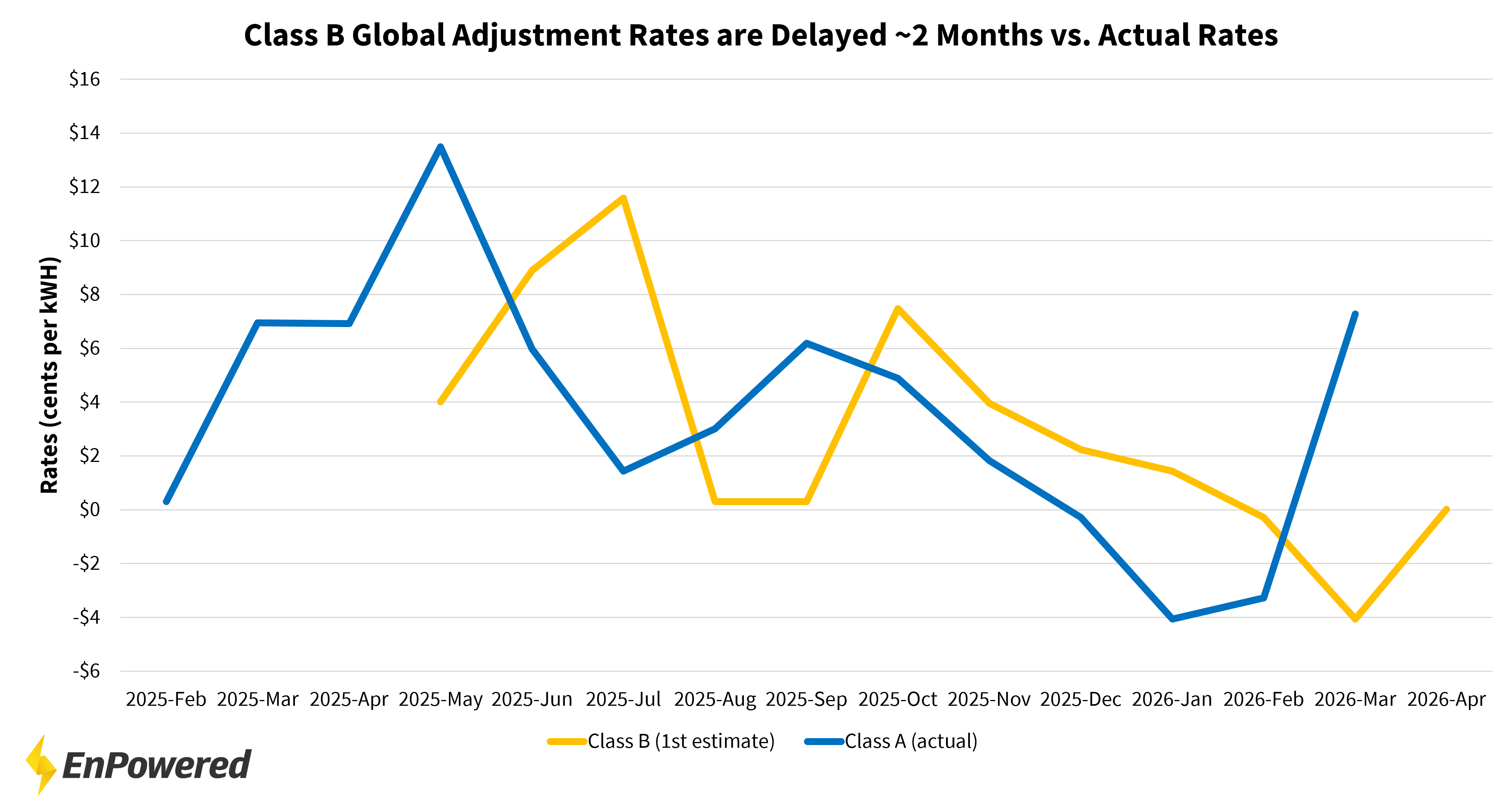
The relationship between Class B and Class A GA rates is rarely as clear as it has been over the last 12 months. As shown in the chart below, the Class B 1st estimate closely mirrors the actual GA rate – but with roughly a two-month delay.
This tells us two important things.
First, over longer periods (like a year), Class A and Class B customers end up paying very similar total GA costs. The system is not structurally biased toward one group or the other.
Second, it means that Class B customers can actually use this relationship to their advantage.
If the actual GA rate today is rising, there is a strong likelihood that the Class B rate will rise in ~2 months. For example, the actual rate in March grew significantly to around 7¢/kWh, so it’s reasonable to expect that the Class B 1st estimate in May will also increase significantly.
This isn’t a perfect predictor, but it’s a useful directional signal.
Why Timing Still Matters
If everything averages out, it’s tempting to conclude that this timing difference doesn’t matter. For many businesses, that’s true. But not for all.
The key factor is seasonality of consumption. Global Adjustment is inversely related to commodity prices. When commodity prices rise – typically during peak summer and winter months – GA tends to fall. Conversely, during shoulder seasons with lower commodity prices, GA tends to increase (for more information on this relationship, read our article here).
For Class A customers, this relationship holds in real time.
For Class B customers, however, that signal is shifted by roughly two months.
This creates an important effect:
- Higher GA costs from shoulder months are pushed into summer and winter
- Lower GA costs from peak months are pushed into shoulder periods
For businesses with relatively flat load profiles, this timing shift has little impact. But for businesses with high seasonal usage, such as facilities with significant summer cooling loads, this delay can result in paying higher GA during periods of highest consumption, increasing total annual costs.
In other words, even though the average rate is similar, when you consume power relative to when costs are incurred starts to matter.
Bottom Line
Class A and Class B Global Adjustment rates are not designed to move together month-to-month. They reflect the same system costs—but at different points in time.
When market conditions shift quickly, as they did this winter, the gap between forecast and reality becomes more visible. But over time, those differences resolve.
For most businesses, this timing difference averages out. But for those with highly seasonal usage, it can create real cost impacts – and opportunities to manage them.

Related Resources